To change the titles text later edit the text in the linked cell rather than on the chart. An axis label is different from an axis title which you can add to describe whats shown on the axis. Axis titles arent automatically shown in a chart. This affects all text labels at the same time. Click on the chart area. 2 In Excel 2013 clicking the Pivot Chart Pivot Chart in the Charts group on the Insert tab. Click anywhere within your Excel chart then click the Chart Elements button and check the Axis Titles box. Add axis titles to a chart When creating graphs in Excel you can add titles to the horizontal and vertical axes to help your users understand what the chart data is about. In the Horizontal Category Axis Labels box click Edit. Select the data you use and click Insert Insert Line Area Chart Line with Markers to select a line chart.
Free Microsoft Excel Training. Adding elements like gridlines labels and data tables help viewers more easily identify whats being presented. To change the titles text later edit the text in the linked cell rather than on the chart. 2 In Excel 2013 clicking the Pivot Chart Pivot Chart in the Charts group on the Insert tab. Now on the vertical axis one change we can make is to use commas for thousands. To learn how to add them see Add or remove titles in a chart. Gridlines are the lines in the background of a chart that correspond to the values in the chart. To add the axes titles for your chart follow these steps. Select the data set Click the Insert tab. To label one data point after clicking the series click that data point.
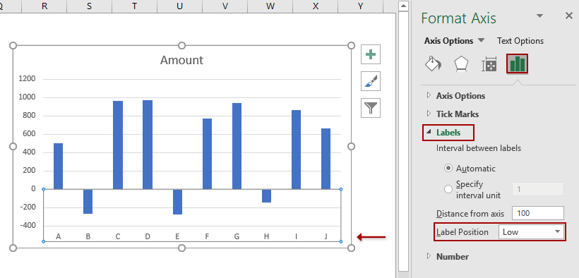
To change the titles text later edit the text in the linked cell rather than on the chart. How To Add Axis Labels In Excel Details. To add the axis titles do the following. In the upper right corner next to the chart click Add Chart Element Data Labels. Finally Ill select the chart and bump up the font size. In the Axis label range box enter the labels you want to use separated by commas. To label one data point after clicking the series click that data point. Add axis titles to a chart When creating graphs in Excel you can add titles to the horizontal and vertical axes to help your users understand what the chart data is about. Select the data you use and click Insert Insert Line Area Chart Line with Markers to select a line chart. To change the location click the arrow and choose an option.
Right click at the axis you want to format its labels as thousandsmillions select Format Axis in the context menu. Show Chart Gridlines. If you are using Excel 2010 you can add a right handside Y axis in a chart as follows. Select the data set Click the Insert tab. Now lets break down what just happened. In the Format Axis dialogpane click Number tab then in the Category list box select Custom and type 999999 MK into Format Code text box and click Add button to add it. Heres how easy and quick it is to add axis titles. To label one data point after clicking the series click that data point. Select the data you use and click Insert Insert Line Area Chart Line with Markers to select a line chart. In the Charts group click on the Insert Columns or Bar chart option.
Click anywhere on the chart you want to add axis labels to. Finally Ill select the chart and bump up the font size. Doing so will cause a group of tabs titled Chart Tools to appear in Excels toolbar with the Design Layout and Format tabs residing within it. Show Chart Gridlines. To change the titles text later edit the text in the linked cell rather than on the chart. In the Axis label range box enter the labels you want to use separated by commas. For example type Quarter 1Quarter 2Quarter 3Quarter 4. The Design and the Format tabs. Add axis titles to a chart When creating graphs in Excel you can add titles to the horizontal and vertical axes to help your users understand what the chart data is about. How to Add Axis Labels to a Chart in Excel How to Display Chart Gridlines Labels and Data Tables in Excel.