Heartwarming Add Border To Excel Chart How Adjust Graph Scale In
How To Set The Border Color And Styles For Excel Chart
Plot a target line with different values. Add a text label for the line. Click that button to open the border menu. Chart Title Border Style and Color in Excel Step 1. Add horizontal benchmarkbasetarget line by adding a new data series in an Excel chart This method will take the benchmark line for example to guide you to add a benchmark line baseline or target line in an existing chart in Excel. Change the line type. Adding borders in Excel 2016Check out my Channel for Dozens more Excel Tutorials. Right click at the chart area and select Format Chart Area from the context menu. This quick example will teach you how to add an average line to a column graph. WithFormatLineVisible msoTrueWeight 05 ForeColorRGB RGB 0 0 205ForeColorRGB RGB 255 0 0Transparency 0 End With It is supposed to add a border around all the bars in the graph red with RGB 25500 blue with RGB 00255.
For accessing borders the shortcut way first selects the data we want to frame with borders and then press ALT H B simultaneously to enable the border menu in Excel.
Extend the line to the edges of the graph area. Add horizontal benchmarkbasetarget line by adding a new data series in an Excel chart This method will take the benchmark line for example to guide you to add a benchmark line baseline or target line in an existing chart in Excel. Display the average target value on the line. Most reports and presentations contain a lot of boring charts that describe the state before and after some event action etc. Right click at the chart area and select Format Chart Area from the context menu. Select the range of cells that you want the gridlines to appear on rows when you enter values.
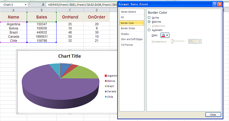
Optional Specify the color of the line that will be drawn around the chart as the border. Since I have used the Excel Tables I get structured data to use in the formulaThis formula will enter 1 in the cell of the supporting column when it finds the max value in the Sales column. To make rounded corners in chart border you need to go to the Format Chart Area dialog first. Add Chart Border in Excel. Plot a target line with different values. Now on the Home tab on the Ribbon youll see a Font section with controls for formatting text. Display the average target value on the line. Change the line type. Right click at the chart area and select Format Chart Area from the context menu. Click Border Styles tab in the Format Chart Area dialog and check Rounded corners option.
Click that button to open the border menu. However as far as I can tell no border is added to any of the bars. In this example I will select the range of cells A1F20. Select the table and insert a Combo Chart. To add borders to cells automatically when you enter data please do with following steps. Double-click on any Excel sheet in your computer to open it up. The Borders button looks like a square with four quadrants. How to add Dividers to the chart. Add a line to an existing Excel chart. Optional Specify the color of the line that will be drawn around the chart as the border.
Most reports and presentations contain a lot of boring charts that describe the state before and after some event action etc. Once we do that we will get a list of all kinds of borders available in excel. Now on the Home tab on the Ribbon youll see a Font section with controls for formatting text. Beside the source data add a Benchmark line column and fill with your benchmark values. Select the table and insert a Combo Chart. Select color you can also edit or adjust other parameters like transparency or width. To have it. Select the range of cells that you want the gridlines to appear on rows when you enter values. However using simple visual tricks you can shake up the audience and draw attention to the essence of your presentation. How to customize the line.
Youll also find a border button that looks like a window a grid of four small boxes. Add Chart Border in Excel. The following screen-shot will show you how to activate a chart title. Add a text label for the line. How to customize the line. Select the cells you want to add all outside borders and then press the Ctrl Shift keys at the same time now you will see the outside borders are added for selected cells immediately. Select Chart Title The first step is to select a chart title to format and change the border styles and color. Double-click on any Excel sheet in your computer to open it up. Extend the line to the edges of the graph area. Add horizontal benchmarkbasetarget line by adding a new data series in an Excel chart This method will take the benchmark line for example to guide you to add a benchmark line baseline or target line in an existing chart in Excel.
Display the average target value on the line. To make rounded corners in chart border you need to go to the Format Chart Area dialog first. ALT H will enable the Home menu B will enable the borders. You can do this by clicking and dragging over the cells you want until they turn blue. Beside the source data add a Benchmark line column and fill with your benchmark values. WithFormatLineVisible msoTrueWeight 05 ForeColorRGB RGB 0 0 205ForeColorRGB RGB 255 0 0Transparency 0 End With It is supposed to add a border around all the bars in the graph red with RGB 25500 blue with RGB 00255. Select the range of cells that you want the gridlines to appear on rows when you enter values. Select Border and click the type of border to apply to the chart. Select the cells you want to add all outside borders and then press the Ctrl Shift keys at the same time now you will see the outside borders are added for selected cells immediately. Right click at the chart and select Format Chart Area in the context menu.