Peerless Add Line Of Best Fit To Scatter Plot In Excel Graph Php Example
How To Add Best Fit Line Curve And Formula In Excel
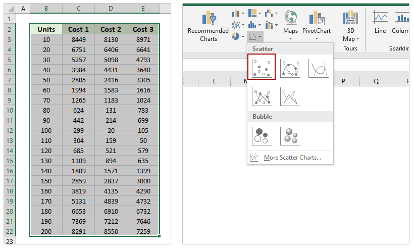
Now it is time to add the Best Fit Line Regression line. Select the down arrow next to it. Step 1 - Open excel type x in cell A1 and type y in cell B1. Occasionally you may want to add a horizontal line to a scatterplot in Excel to represent some threshold or limit. To add the Trendline click on any blank space within the scatter graph. Learn to create and format a scatter plot and line of best fit using Excel 2007. Select the original experiment data in Excel and then click the Scatter Scatter on the Insert tab. Add a line of best fit through the data here. Scatterplots and correlation in Excel statstutor community project wwwstatstutoracuk Correlation. Chart menu Add Trendline is the command that will be available when you have a Chart selected or when a Chart worksheet is the active worksheet.
If you choose Linear then Excel give you the best fit for the data based on a linear response.
We can then select any desired trendline that match our scatter plot. Estimate a first degree polynomial using the same x values and add to the ax object created by thescatter plot. Creating a Line of Best FitStandard Curve on Excel 2013. Look for the icon of a graph with just dots on it. 05-21-2012 at 1209 PM. Select Insert in the main toolbar.
See above screen shot. Follow up to receive email notifications. We can then select any desired trendline that match our scatter plot. To add the Trendline click on any blank space within the scatter graph. Next click anywhere on the scatterplot. Learn to create and format a scatter plot and line of best fit using Excel 2007. Step 1 - Open excel type x in cell A1 and type y in cell B1. This is what Excel calls a best fit line. In this case we stick with Linear Trendline because we think it is the best fit line excel provides for our type of data. Select the new added scatter chart and then click the Trendline More Trendline Options on the Layout tab.
Next click anywhere on the scatterplot. To add the Trendline click on any blank space within the scatter graph. Last edited by ChemistB. You can use nppolyfit and nppoly1d. Select the new added scatter chart and then click the Trendline More Trendline Options on the Layout tab. Next highlight the data in the cell range A2B17 as. He means duplicate all the data you want on the graph in your spreadsheet in an added column to the table with the exception of the points you wish to exclude. Select the original experiment data in Excel and then click the Scatter Scatter on the Insert tab. Occasionally you may want to add a horizontal line to a scatterplot in Excel to represent some threshold or limit. Chart Layouts section will appear on the Ribbon.
Select Insert in the main toolbar. Select the down arrow next to it. Learn to create and format a scatter plot and line of best fit using Excel 2007. This will automatically add a simple linear regression line to your scatterplot. If you choose Linear then Excel give you the best fit for the data based on a linear response. You can use nppolyfit and nppoly1d. Estimate a first degree polynomial using the same x values and add to the ax object created by thescatter plot. Right Click on any one of the data points and a dialog box will appear. Add a line of best fit through the data here. Best fit line without outliers.
Best fit line without outliers. Creating a Line of Best FitStandard Curve on Excel 2013. Chart menu Add Trendline is the command that will be available when you have a Chart selected or when a Chart worksheet is the active worksheet. First lets create the following fake dataset. Select the new added scatter chart and then click the Trendline More Trendline Options on the Layout tab. Select Insert in the main toolbar. 05-21-2012 at 1209 PM. Add a Regression Line. Select the first scatter graph with just dots and no lines. If you choose Linear then Excel give you the best fit for the data based on a linear response.
Step 2 - Enter seven values for x in column A. Chart menu Add Trendline is the command that will be available when you have a Chart selected or when a Chart worksheet is the active worksheet. Next click anywhere on the scatterplot. Then when you format your chart area make a scatter plot of both sets of data but only add a trendline for the duplicated set. Last edited by ChemistB. Learn to create and format a scatter plot and line of best fit using Excel 2007. Chart Layouts section will appear on the Ribbon. Excel will be used to create the values from the equation will then be used to display a scatter plot of the data and then will be used to find the best fit for the given data. We will click on Chart Layout under the Charts tab and select Trendline. This tutorial provides a step-by-step example of how to quickly add a horizontal line to any scatterplot in Excel.