Select Regression and click OK. On the top ribbon click the INSERT tab then click INSERT Scatter X Y or Bubble Chart in the Charts group and click. Most statistical texts show the correlation coefficient. Once you click on Data Analysis a new window will pop up. The regression line is. Creating a linear regression line trendline Using the regression equation to calculate slope and intercept. Click on Insert and expand the dropdown for Scatter Chart and select Scatter thumbnail first one Now a scatter plot will appear and we would draw the regression line on this. If you dont see this option then you need to first install the free Analysis ToolPak. It produces an equation where the coefficients represent the relationship between each independent variable and the dependent variable. To add a regression line choose Layout from the Chart Tools menu.
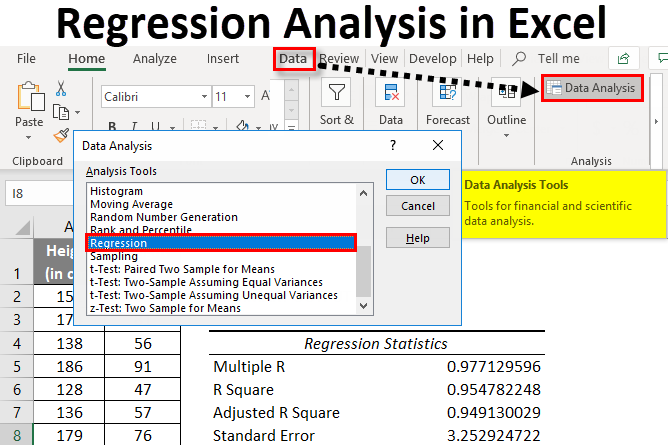
Select the Input Y Range which is your dependent variable. Scroll down to find the regression option and click OK. This add-in enables Excel to perform difficult statistical analysis but it is not enabled by default in Excel installations. Select Regression and click OK. On the top ribbon click the INSERT tab then click INSERT Scatter X Y or Bubble Chart in the Charts group and click. On the Data tab in the Analysis group click the Data Analysis button. To draw the regression line lets add a trendline on the chart. Simply click on your scatter plot from the Ribbon select Chart Tools Design Add Chart Element Trendline Linear Your trendline appears on your chart. If you dont see this option then you need to first install the free Analysis ToolPak. Regression analysis describes the relationships between a set of independent variables and the dependent variable.
Regression analysis describes the relationships between a set of independent variables and the dependent variable. The final method for performing linear regression in Excel is to use the Analysis Toolpak add-in. Select the Linear TrendRegression type. In the dialog box select. Linear Regression in Excel-2007 Table of Contents. On the top ribbon click the INSERT tab then click INSERT Scatter X Y or Bubble Chart in the Charts group and click. To run the regression arrange your data in columns as seen below. This tutorial provides a step-by-step example of how to quickly add a simple linear regression line to a scatterplot in Excel. First lets create a simple dataset to work with. Performing a simple linear regression in Excel is ridiculously easy.
This is valuable information. Select the two columns of the dataset x and y including headers. Multiple Regression Analysis in Excel. Scroll down to find the regression option and click OK. A dialogue box appears Figure 2. Creating a linear regression line trendline Using the regression equation to calculate slope and intercept. On the Data tab in the Analysis group click the Data Analysis button. Once you click on Data Analysis a new window will pop up. Select the down arrow next to it. Look for the icon of a graph with just dots on it.
Click on any of the data points and right-click. To run the regression arrange your data in columns as seen below. Select the Input Y Range which is your dependent variable. In the dialog box select. Next highlight the cell range A2B21. Scroll down to find the regression option and click OK. Most statistical texts show the correlation coefficient. I personally find the line. Learn how to create a regression line for your chart in Excel. Create an initial scatter plot.