Peerless Excel Chart Add Threshold Line R Horizontal Bar

This will select the line and open the Format Data Series pane on the right side of your Excel window. Reselect the data series and now change series chart type to line. You know have TWO columns. Adding a series data. To achieve this effect add a line to your chart as explained in the previous examples and then do the following customizations. Select the entire table and insert a line chart with markers. In that box that pops up click the Add button to add a new series. I create the graphs in excel and paste in the. Itll look like this but dont freak out. Then right-click on the graph and click Select Data.

Next right click anywhere on the chart and click Select Data. Go Design tab chart layouts group add chart element dropdown data labels center. Add the cell or cells with the goal or limit limits to your data for example. Add the date with the current date to your data for example. Add a static threshold line to a chart. Select the entire table and insert a line chart with markers. Hover over the bottom right corner and click and drag the highlighted area of the table to extend the selection to the column Target. In your graph double-click the target line. Under Chart Tools on the Design tab. Add horizontal benchmarkbasetarget line by adding a new data series in an Excel chart This method will take the benchmark line for example to guide you to add a benchmark line baseline or target line in an existing chart in Excel.

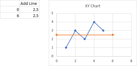
The resulting line extends to the edges of the plotted area but Excel changed the Axis Position to Between Tick Marks. Edit Series preview pane. Click the chart title and then select Edit. Itll look like this but dont freak out. I am creating a powerpoint pres and in which I am copy pasting graphs from an excel sheet. Get the sample file here. Get Your Free Trial. Under Chart Tools on the Design tab. Right click on the added series and change its chart type to XY Scatter With Straight Lines And Markers again the markers are temporary. In that box that pops up click the Add button to add a new series.

First of all select the data table and insert a column chart. Eg this will be useful to show data and highlight a current date. Sometimes you need to add a horizontal line to your chart. This will put 15 as the data label. In the Value field type a number that indicates the threshold value for the line. Click Add under Legend Entries. Get Your Free Trial. In that dialogue box select your Benchmark data. The easiest way to get these new data in the chart is to double-click into the chart area to highlight all the data already shown in the graph. The Select Data Source dialog box will pop-up.

In the Value field type a number that indicates the threshold value for the line. Under Chart Tools on the Design tab in the Data group choose Select. Right click on the added series and change its chart type to XY Scatter With Straight Lines And Markers again the markers are temporary. The techniques for adding datum lines to charts rely on the ability to use combination charts. To add a horizontal line to your chart do the following. Click the Analysis tab. Left click on the data label twice see the selection box has four squares in four corners of selection and go to the format tab. Reselect the data series and now change series chart type to line. The Select Data Source dialog box will pop-up. The easiest way to get these new data in the chart is to double-click into the chart area to highlight all the data already shown in the graph.