Under Chart Tools on the Format tab in the Current Selection group click the arrow next to the Chart Elements box and then click the chart element that you want to use. The bottom line is that it all depends on the chart type the chart type mix and the distribution of chart series between primary and secondary axis. Change Fill to No Fill. Keep in mind that that you dont have reverse the axis in a case like this. Sort it in reverse order ie. The Format Axis task pane opens. Right click the axis you want to change select Format Axis from context menu. On the Format tab in the Current Selection group click Format Selection. The data is sorted in descending order Then I added. In the Axis Labels dialog box change the Axis label range field by deleting everything to the right of the exclamation mark and replacing it with the named range Comp.
In the Axis Labels dialog box change the Axis label range field by deleting everything to the right of the exclamation mark and replacing it with the named range Comp.
See screen shot below. To reset the axis to its default visit axis options again and set the axis crossing to automatic and untick the reverse order checkbox. Click Data tab and go to Sort Filter group and select the sort order you need. Now you can see the data has been sorted and the chart. One way to solve the problem is to add a another column to the data table with ranking numbers the way you want to sort it. In the Format Axis pane in the right click the Axis Options button and change the number in the Major box in the Units section.
Under Chart Tools on the Format tab in the Current Selection group click the arrow next to the Chart Elements box and then click the chart element that you want to use. There a couple of ways to change chart plot order the order that Excel plots data in a chart. Step 6 Deselect Chart Title and Legend in Chart Elements. On the Format tab in the Current Selection group click Format Selection. To create a column chart execute the following steps. In the Select Data Source dialog box in the Horizontal Category Axis Labels zone click Edit. Then go to the Select data after right-click on the chart and overwrite the range with the named formula. Right click the axis you want to change select Format Axis from context menu. To reset the axis to its default visit axis options again and set the axis crossing to automatic and untick the reverse order checkbox. Sound like a silly question but it is a bit confusing indeed.
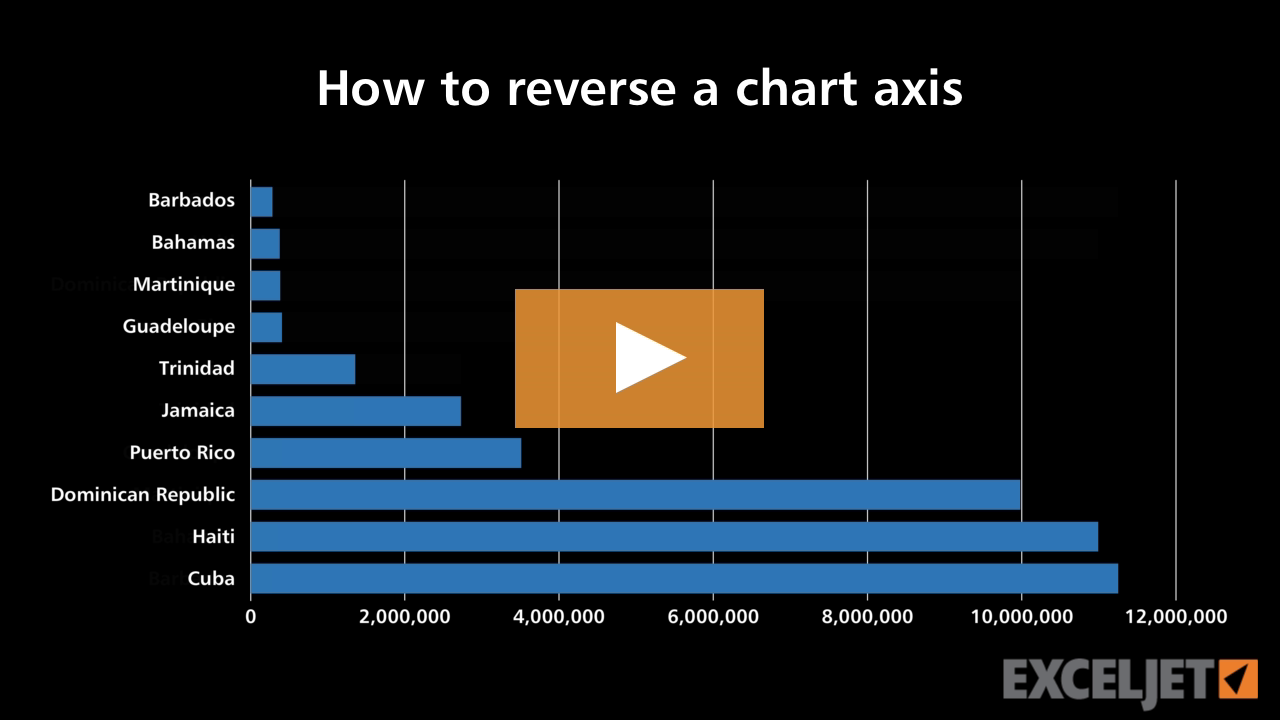
In the Axis Options category under Axis Options select the Series in reverse order check box. In the Axis Labels dialog box change the Axis label range field by deleting everything to the right of the exclamation mark and replacing it with the named range Comp. Right click the axis you want to change select Format Axis from context menu. To reset the axis to its default visit axis options again and set the axis crossing to automatic and untick the reverse order checkbox. You will have to manually drag the fields to provide sorting order. Sort it in reverse order ie. Click the DESIGN tab on the Ribbon. Then in the popped out dialog make sure the Expand the select is checked and click Sort button. In the Select Data Source dialog box in the Horizontal Category Axis Labels zone click Edit. Ill show you two examples in Excel Video 471.
The bottom line is that it all depends on the chart type the chart type mix and the distribution of chart series between primary and secondary axis. One day a friend asked me how to sort a bar chart in descending order. On the Format tab in the Current Selection group click Format Selection. Click the DESIGN tab on the Ribbon. You can always sort. Click Data tab and go to Sort Filter group and select the sort order you need. To reset the axis to its default visit axis options again and set the axis crossing to automatic and untick the reverse order checkbox. In Excel you can apply Custom Sort on a range table. In the Axis Options section click the Axis Options icon if necessaryit looks like a graph check the Categories in Reverse Order check box. In the Format Axis pane in the right click the Axis Options button and change the number in the Major box in the Units section.
Under Chart Tools on the Format tab in the Current Selection group click the arrow next to the Chart Elements box and then click the chart element that you want to use. A horizontal axis or x-axis and a vertical axis or y-axis. Sound like a silly question but it is a bit confusing indeed. Click Data tab and go to Sort Filter group and select the sort order you need. There a couple of ways to change chart plot order the order that Excel plots data in a chart. Under Chart Tools on the Format tab in the Current Selection group click the arrow next to the Chart Elements box and then click the chart element that you want to use. Now you can see the data has been sorted and the chart. Simply highlight the values on the sheet and insert the chart you would like to use. Sort it in reverse order ie. Change Fill to No Fill.
Then in the graph add that column to the Tooltips field on the right bar. Next you have to create the Whiskers. To create a column chart execute the following steps. In the Axis Labels dialog box change the Axis label range field by deleting everything to the right of the exclamation mark and replacing it with the named range Comp. I told her to sort the data. Sound like a silly question but it is a bit confusing indeed. Normally the best way to influence the order of the legend items is to sort the data table and re-arrange the order of the rows or columns respectively. This example teaches you how to change the axis type add axis titles and how to change the scale of the vertical axis. Keep in mind that that you dont have reverse the axis in a case like this. Step 6 Deselect Chart Title and Legend in Chart Elements.