The typical dynamic range chart advice is to use a table where the chart expands when more data is. With the chart selected go to the Design tab. That is where you will want to create a chart with a dynamic range. By default Microsoft Office Excel determines the minimum and maximum scale values of the vertical value axis also known as the y axis when you create a chart. Excel also shows the dates between 8242018 and 91 2018. Axis Scale Parameters in the Worksheet You need a place to put the axis scale parameters. At the top of the window select the Layout tab and then click the Axis button. Click the Excel file where the graph is located and click on the graph. 2 Excel refers to this type of histogram chart as Column charts. Select the Y-Axis Right-Click the highlighted Y-Axis and select Format Axis.
However there are times when you want to provide you ow. With the chart selected go to the Design tab. Select the Y-Axis Right-Click the highlighted Y-Axis and select Format Axis. When creating a chart most of the time youd take the default axis labels that Excel would provide. A standard chart in Excel uses a defined set of cells for the category axis and the data values. Sub Axis Dim Cht As ChartObject Set Cht WorksheetsData Input SummaryChartObjectsChart 2Chart With ChtAxesxlCategory MaximumScale RangeZ7Value MinimumScale RangeZ6Value End With With ChtAxesxlValue MaximumScale RangeZ9Value MinimumScale Range. Excel also shows the dates between 8242018 and 91 2018. Right click the axis you want to change select Format Axis from context menu. Open the Format tab and select Format Selection Go to the Axis Options click on Number and select Number from the. Go to the Insert tab.
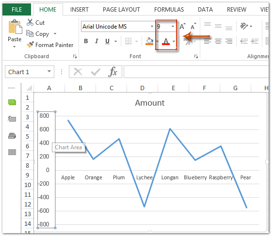
Dim yax As Axis Set yax chtChartAxes xlValue yaxMinimumscale 100 Now works everything well. Public object Axes object Type MicrosoftOfficeInteropExcelXlAxisGroup AxisGroup MicrosoftOfficeInteropExcelXlAxisGroupxlPrimary. Click on the axis that you want to customize. Click on Insert Line or Area Chart and insert the Line with markers chart. The format Axis prompt box will open. This works for most charts. From the menu Make sure you are within the Axis Options section of the Format Axis Pane Within the Bounds section manually input your Minimum and Maximum axis limits. This example can be expanded to include secondary axes or to change other charts as well. Go to the Insert tab. In series values change range reference with named range amount.
When creating a chart most of the time youd take the default axis labels that Excel would provide. With the chart selected go to the Design tab. The Format Axis pane appears. An easier way to make the chart dynamic is by converting the source range to a table and to specify the table as chart data range. Go to the Insert tab. At the top of the window select the Layout tab and then click the Axis button. Sub Axis Dim Cht As ChartObject Set Cht WorksheetsData Input SummaryChartObjectsChart 2Chart With ChtAxesxlCategory MaximumScale RangeZ7Value MinimumScale RangeZ6Value End With With ChtAxesxlValue MaximumScale RangeZ9Value MinimumScale Range. Click on the axis that you want to customize. To remove these dates change the axis type from Date axis to Text axis. Instead of the Excel style range notation you can use the following list syntax which is easier to create programmatically.
See screen shot below. Click on Insert Line or Area Chart and insert the Line with markers chart. This works for most charts. The format Axis prompt box will open. Right click on your chart and select Select Data. By default Microsoft Office Excel determines the minimum and maximum scale values of the vertical value axis also known as the y axis when you create a chart. In the Format Axis pane in the right click the Axis Options button and change the number in the Major box in the Units section. Open the Format tab and select Format Selection Go to the Axis Options click on Number and select Number from the. At the top of the window select the Layout tab and then click the Axis button. The typical dynamic range chart advice is to use a table where the chart expands when more data is.